Following on from previous posts this post will look at the specific variations of formatting that can be applied to blank cells to ensure consistency through cells containing the same data type and also to ensure the worksheet is displaying data in the format you prefer to use.
TOP TIP: To format whole columns without including your headings highlight a minimum of 2 cells then hold down CTRL + SHIFT and press the ↓
Format Number
On this post we will be exploring the Format Number tab when formatting cells in order to apply specific formats
- Select the Column, Row or selection of cells you wish to apply the formatting to
- From the Home Tab select Format > Format Cells
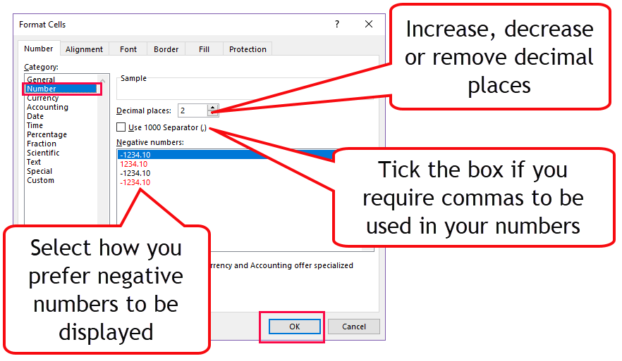
- From the Number Tab select the required category (see below)
General
General is the formatting style that is automatically applied to all cells by default. Formatting will change the appearance of the data based on how it is entered. See previous blog posts for more detailed information.
Number
Number ensures data entered is treated as a number, however you can determine how you want to specifically have that data look here.
Negative numbers can be displayed with or without a minus and or in red text.
Currency
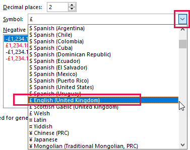
Currency has similar settings as Number (see above) however you are able to also select the currency symbol of you choice.
- Click on the drop down list and select accordingly
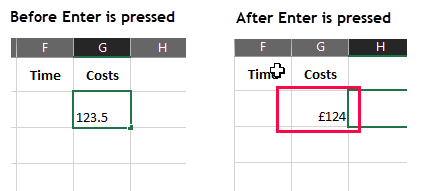
Example: No matter how you enter your data into the field it will display as the format chosen i.e. £ English (UK) with no decimal places (even if decimals are entered Excel will round up based on the formatting setting applied)
Accounting
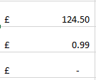
Applies currency options as above however it will place the currency symbol aligned left and the data aligned right. Anything with a 0 entry will be replaced with a – (dash)
Date
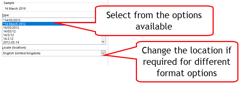
Formatting can be applied to dates as long as excel recognised that the data entered is a date:
Recognised entry formats would be:
containing / or –
text entry i.e. 12 Mar 18
If only partial date is entered then Excel will format based on the format settings and the information to hand i.e. if 12/18 is entered in a cell formatted to display a full date with the month in text Excel will default to the 1st of the month (01 December 2018)
If dates are entered into a date formatted cell in an unrecognised date format then it will convert the cell to text e.g. 01.12.18 will remain as this but Align to the left. To avoid this you can apply validation to ensure the data is entered in a specific format. We will cover this is a future post.
Time
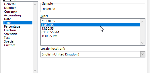
Time behaves in a similar way to Date in that it must be entered in the appropriate way in order to be formatted correctly. As with date you may need to use a combination of validation and formatting to get the optimum results.
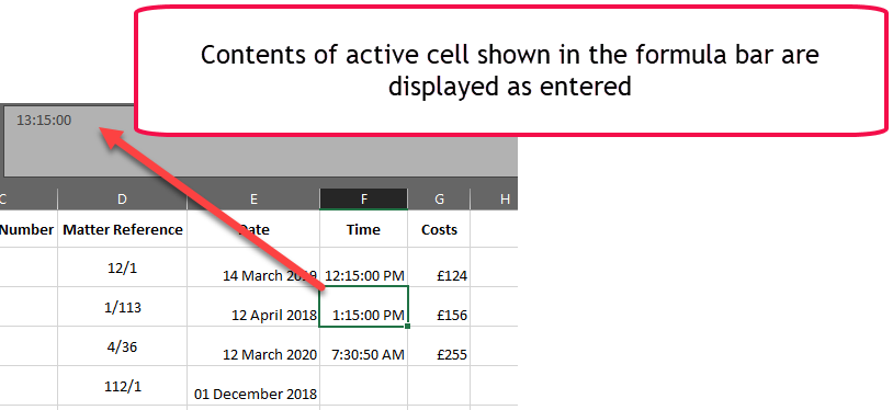
Time should always be entered using : (colon) to separate hours, minutes and seconds and in 24 hour clock format.
The default options show hours, minutes and seconds in variations of 24hr or AM/PM. To produce a different time format you may need to use the custom format (we will cover this in the next post)
Example of format so far:
The next blog posts will further explore the options in the Format tab including Percentage, Fraction, Text and Custom.
If you would like any specialised training for any area of Excel please get in touch with the training team at Fusion to discuss.
Sharon Brook – IT Training Manager – 01484 500767 – [email protected]


