Formatting Blank Cells
By formatting blank cells you can force the data that is entered to be formatted how you would like it.
See below examples of how data can look when entered on both an unformatted and formatted worksheet.
Setting Formatting
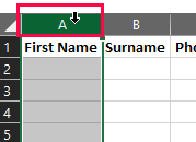
Select either the entire row/column or cells you wish to format
- To format column A click on the number header you will see a small black arrow. This will then highlight the entire column.
- Repeat for all other columns. You can also select more than one column at a time in order to apply the same formatting.
- Eg. in this example we could select both column A and B to apply the same sort of text formatting.
With a single or multiple columns/rows selected, formatting can now be applied to the cells.
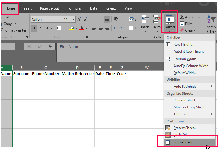
- Select Home Tab
- Click Format
- Select Format Cells
Format Cells
in the Format Cells window there are several tabs to use for formatting. In this post we will only cover those relating to data content and not design i.e. Number, Alignment and Font
Number
The number tab will allow you to select the type of data you wish to be displayed in a cell, please refer to the previous blog post Excel – Producing Consistent Data for details of excels default selections
The table below briefly describes what each option on the number tab will do to your data.
You will see within each option there are further more detailed formats you can apply we will cover these in more depth in future posts.
- Select the appropriate option and that will apply to your cell.
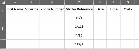
e.g. in the Matter Reference column shown in the image below we would want to ensure that when entering this data as 12/11 that excel does not change this to a date format.
- Select the column to format and proceed to the Format Cells/Number Tab as shown above.
- Choose the Text option
Data will now appear as shown
Alignment
The Alignment Tab will allow you to change the default alignment of data within a cell to enable better layout and readability of worksheets.
- Select the column/rows to be formatted
- Select Format Cells as above
- Click on Alignment Tab
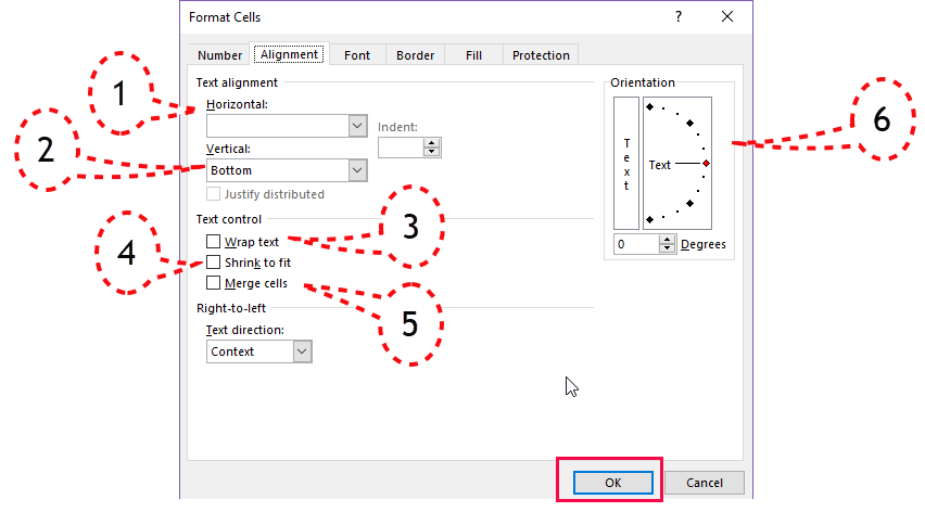
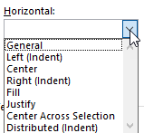
1 Horizontal Alignment
- Select the position of the data horizontally across the cell.
- Click on the drop down list and choose from the selection
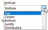
2 Vertical Alignment
- Select the position of the data vertically up/down the cell
- Click on the drop down list and choose from the selection.
3 Wrap Text
- ensure the data will wrap around the current width of the cell, ensuring all text is displayed, automatically altering the height of the cell if required.
4 Shrink to Fit
- Data will shrink in text size to fit the current width of the cell to ensure all text is displayed.
5 Merge Cells
- Cells can be merged to make one cell across multiple columns or rows. NB: all cell restrictions will still apply, this is still only one cell it does not increase its text capacity.
6 Orientation
- Data can be displayed at angles, vertically or horizontally. Adjustments may need to be made to cell height and width to allow for data to be properly displayed.
Example below shows cell formatted to display data centred horizontally and vertically.
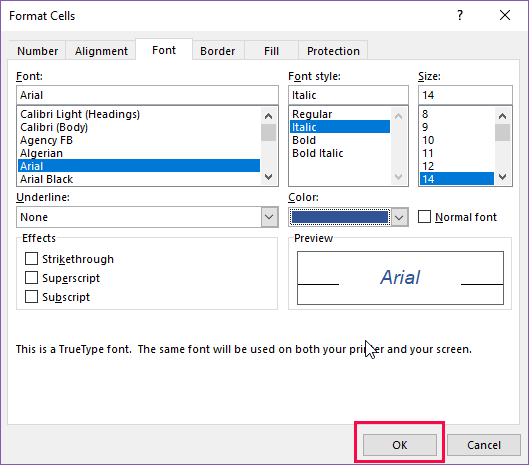
Font
You can format the font of selected cells, columns, rows or the entire worksheet.
- Click to select the Font
- Select Font Style
- Select Font Size
- Select Underline
- Select Font Colour
All or any of the above can be used to help enhance your worksheet
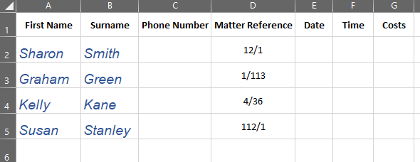
The example below shows the Name columns formatted to display Arial Italic 15 in Blue
The next posts will cover the specific formats within the Numbers format tab. This will cover date formats, number formats, time and currency plus custom formats.
If you would like any specialised training for any area of Excel please get in touch with the training team at Fusion to discuss.
Sharon Brook – IT Training Manager – 01484 500767 – [email protected]


