This post is a continuation from our last blog about Detailed Formatting in Excel.
In this post we will look at the remaining options on the Format Cells>Number Tab
Format Number
We will be exploring the Format Number tab when formatting cells in order to apply specific formats from Percentage to Custom
- Select the Column, Row or selection of cells you wish to apply the formatting to
- From the Home Tab select Format > Format Cells
- From the Number Tab select the required category (see below)
Percentage
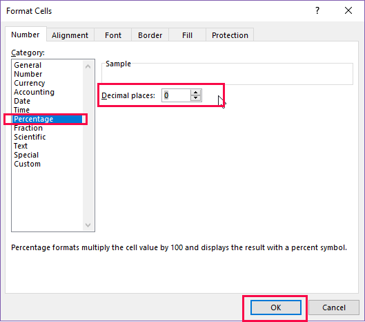
To apply a percentage format to your worksheet
- Select as above
- Click Percentage
- Choose whether decimal places are required and if so how many.
- Click OK
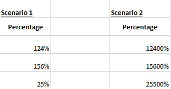
Percentage format will multiply the cell value by 100 and display the result with a percent symbol. This can have different outcomes depending on if you are formatting blank cells and then inputting data or if the data is there and you then apply the format the results will be different.
Example: In Scenario 1 the blank cells were formatted to percentage prior to entry. In scenario 2 the data was already entered and then the percentage format was applied after.
Fraction
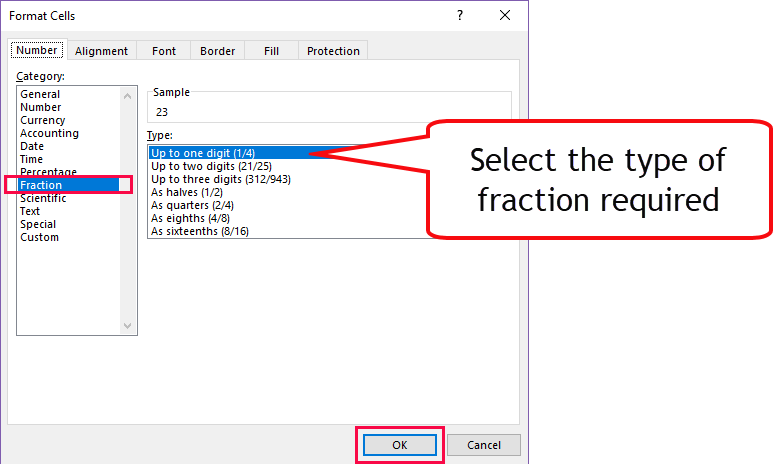
You can use Fraction to ensure that the data entered is converted from a decimal entry to a fraction figure.
The results are as shown
Text
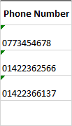
Cells formatted as Text will display entered data as text. If a number has a leading 0 then this will be retained as the data is not formatted as a number.
As you can see from the example shown below the data is now aligned to the left of the cell not the right as numbers are defaulted to.
Custom
Custom option for formatting allows you to customise formatting on certain format types
Custom options can be used for everything however they work particularly well on dates and times
Example 1 – Currency
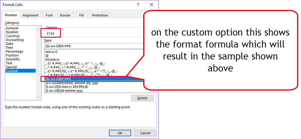
This shows how you can customise a currency format to move your £ symbol to align to the left an the numbers to the right .
This can be changed and customised to your own specification by typing the required format formula into the Type field as shown below:
this is the result
Example 2 – Dates
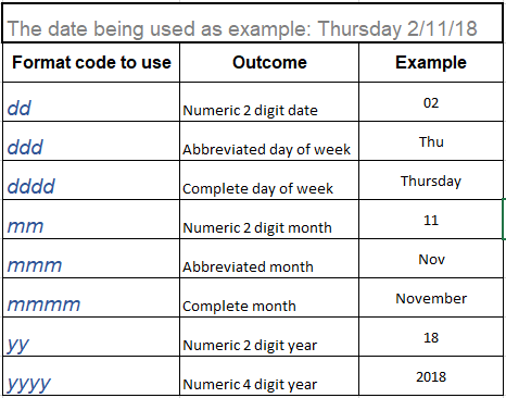
In example 2 we will see how easy it is to customise date fields by following a simple code:
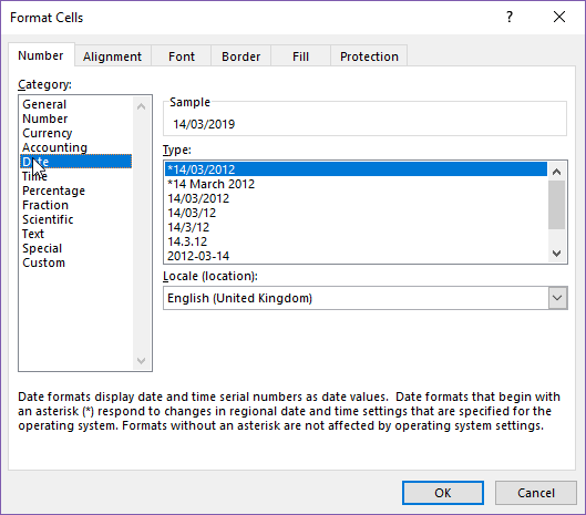
When selecting a date format you can see the options displayed and how they will appear
When you choose to change the date using the Custom options you can see the date formats are displayed in a text format style so you will be required to follow the table above in order to produce your date exactly as you would like.
The following example will shows how to format the field to achieve this format : Thursday 02 November 2018
You will only need to enter 2/11/18 in order for the above to appear if formatted correctly.
Example 3 – Time
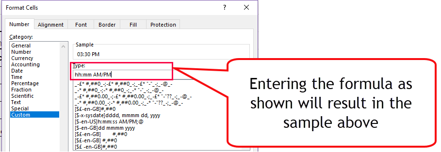
Customising time formats works in the same way as dates above. All times should be entered as 24 hour clocks but then you can use the format codes shown below to format the field accordingly.
Type in the required format code and select OK when complete.
Please note that within your field you can actually use combinations of these custom format codes in order to achieve varying results:
if you enter 16:40 22/6/18 in a cell that is custom formatted as hh:mm AM/PM dddd dd mmmm yyyy. The formatted data will appear as 4:40 PM Friday 22 June 2018.
Try typing combinations of codes within the type field as previously shown and check the Sample to see how it will appear so you do not have to keep re-formatting until it is correct.
The next blog posts will look at validating fields to prevent incorrect data entry.
If you would like any specialised training for any area of Excel please get in touch with the training team at Fusion to discuss.
Sharon Brook – IT Training Manager – 01484 500767 – [email protected]


